3D N-Body Pendulum
Note
You can download this example as a Python script:
3d-n-body-pendulum.py or Jupyter notebook:
3d-n-body-pendulum.ipynb.
Objectives
Show how to use
pydy.vizto generate a 3D animation.Show how to use a non-default ODE_solver.
Show how to calculate noncontributing forces.
Show how to calculate the energies of the system and plot them.
Description
A pendulum consisting of three rods of length \(l\) and mass
\(n_{\textrm{link}}\).
A ball of mass \(m\) and radius \(r\) is attached to each rod, such
that the rod goes through the center of each ball. The center of the ball is
fixed at the middle of the rod. The ball rotates around the rod. If two balls
collide, they are ideally elastic, with spring constant \(k\).
The collision is modeled using the sm.Heaviside(..) function.
The balls are ideally slick, so collisions will not affect their rotation.
There may be speed dependent friction between
the rod and the ball, with coefficient of friction \(\textrm{reibung}\).
A particle with mass \(m_1\) is attached to each ball.
import sympy as sm
import sympy.physics.mechanics as me
import numpy as np
import matplotlib.pyplot as plt
from scipy.integrate import solve_ivp
from pydy.system import System
from pydy.viz.shapes import Cylinder, Sphere
from pydy.viz.scene import Scene
from pydy.viz.visualization_frame import VisualizationFrame
Equations of Motion, Kane’s Method
m, m1, m_link, g, r, l, reibung, k, t = sm.symbols(
    'm, m1, m_link, g, r, l, reibung, k, t')
iXX, iYY, iZZ = sm.symbols('iXX, iYY, iZZ')

N = me.ReferenceFrame('N')  # inertial frame
P0 = me.Point('P0')         # Point fixed in N
t = me.dynamicsymbols._t

q = [me.dynamicsymbols('q' + str(i) + j) for i in range(3)
    for j in ('x', 'y', 'z')]     # holds the gen. coords of each rod
u = [me.dynamicsymbols('u' + str(i) + j) for i in range(3)
    for j in ('x', 'y', 'z')]     # generalized angular speeds

A = [me.ReferenceFrame(f'A{i}') for i in range(3)]   # frames of each link

# geometric center of each body
Dmc = [me.Point(f'Dmc{i}') for i in range(3)]

# mass center of each link
Dmc_link = [me.Point(f'Dmc_link{i}') for i in range(3)]

# points at end of each rod. Dmc_i is between P_i and P_i+1
P = [me.Point(f'P{i}') for i in range(3)]

# marks a red dot on each ball, just used for animation
punkt = [me.Point(f'punkt{i}') for i in range(3)]
The lists rot, rot1 are used for the kinematical equations, see below.
rot = []
rot1 = []
It is useful that the angular speeds be expressed in terms of the ‘child frame’, otherwise the equations of motion become very large.
A[0].orient_body_fixed(N, (q[0], q[1], q[2]), '123')
rot.append(A[0].ang_vel_in(N))
A[0].set_ang_vel(N, u[0]*A[0].x + u[1]*A[0].y + u[2]*A[0].z)
rot1.append(A[0].ang_vel_in(N))

for i in range(1, 3):
    A[i].orient_body_fixed(A[i-1], (q[3*i], q[3*i+1], q[3*i+2]), '123')
    rot.append(A[i].ang_vel_in(N))
    A[i].set_ang_vel(N, u[3*i]*A[i].x + u[3*i+1]*A[i].y + u[3*i+2]*A[i].z)
    rot1.append(A[i].ang_vel_in(N))
Set virtual speeds and noncontributing forces.
auxx, auxy, auxz, fx, fy, fz = me.dynamicsymbols('auxx auxy auxz fx fy fz')
Locate the various points, and define their speeds. Add the virtual speeds to the suspension point P[0].
P[0].set_pos(P0, 0)
P[0].set_vel(N, auxx * N.x + auxy * N.y + auxz * N.z)  # Virtual speeds.
Dmc[0].set_pos(P[0], l/2. * A[0].y)
Dmc_link[0].set_pos(P[0], l/2. * A[0].y)
Dmc_link[0].v2pt_theory(P[0], N, A[0])
Dmc[0].v2pt_theory(P[0], N, A[0])
punkt[0].set_pos(Dmc[0], r*A[0].z)  # only for the red dot in the animation
punkt[0].v2pt_theory(Dmc[0], N, A[0])

for i in range(1, 3):
    P[i].set_pos(P[i-1], l * A[i-1].y)
    P[i].v2pt_theory(P[i-1], N, A[i-1])
    Dmc[i].set_pos(P[i], l/sm.S(2.) * A[i].y)
    Dmc[i].v2pt_theory(P[i], N, A[i])
    Dmc_link[i].set_pos(P[i], l/sm.S(2.) * A[i].y)
    Dmc_link[i].v2pt_theory(P[i], N, A[i])
    punkt[i].set_pos(Dmc[i], r*A[i].z)
    punkt[i].v2pt_theory(Dmc[i], N, A[i])
Make the list of the bodies.
iXX = 2.0 / 5.0 * m * r**2
iYY = iXX
iZZ = iXX

balls = []
points = []
links = []
for i in range(3):
    Inert = me.inertia(A[i], iXX, iYY, iZZ)
    balls.append(me.RigidBody('body' + str(i), Dmc[i], A[i], m,
                          (Inert, Dmc[i])))
    # the red dot may have a mass
    points.append(me.Particle('punct' + str(i), punkt[i], m1))
    inert_link = me.inertia(A[i], m_link*l**2/12., 0, m_link*l**2/12.)
    links.append(me.RigidBody('link' + str(i), Dmc_link[i], A[i], m_link,
                              (inert_link, Dmc_link[i])))
bodies = balls + points + links
Set up the forces.
There are:
potential gravitational forces
potential spring forces when the balls penetrate each other
dissipative friction forces due to friction between rods and balls, if \(\textrm{reibung} \neq 0\)
FG = ([(Dmc[i], -m*g*N.y) for i in range(3)] +
      [(punkt[i], -m1*g*N.y)for i in range(3)] +
      [(Dmc_link[i], -m_link*g*N.y) for i in range(3)])

FB = []
for i in range(3):
    for j in range(i+1, 3):
        aa = Dmc[j].pos_from(Dmc[i])
        bb = aa.magnitude()
        aa = aa.normalize()
        forceij = (Dmc[j],  k * (2 * r - bb) * aa *
                   sm.Heaviside(2 * r - bb))
        FB.append(forceij)
        forceji = (Dmc[i], -k * (2 * r - bb) * aa *
                   sm.Heaviside(2 * r - bb))
        FB.append(forceji)

    friction_i = (A[i], -reibung * u[3*i + 1] * A[i].y)  # around A[i].y
    FB.append(friction_i)

loads = FG + FB
Add the noncontributing forces (here: reaction forces) to the list of forces.
loads += [(P[0], fx * N.x + fy * N.y + fz * N.z)]
Kinematic equations.
Again it is advantageous that the frames A[i] be used below. Otherwise the equations of motion become large. Note how rot, rot1 from above are used.
kd = []
for i in range(3):
    for uv in A[i]:
        kd.append(me.dot(rot[i] - rot1[i], uv))
Finish Kanes’s equations.
q1 = q
u1 = u
aux = [auxx, auxy, auxz]

KM = me.KanesMethod(
    N,
    q_ind=q1,
    u_ind=u1,
    kd_eqs=kd,
    u_auxiliary=aux,
    bodies=bodies,
    forcelist=loads,
)
fr, frstar = KM.kanes_equations()
Numerically Integrate the Equations of Motion
Create a specific ODE solver.
def ode_solver(f, x0, ts, args=(), **kwargs):
    return solve_ivp(lambda t, x: f(x, t, *args), ts[[0, -1]], x0,
                 t_eval=ts, **kwargs).y.T
Initialize an instance of System. If an ODE solver is specified, it must be passed to the System at initialization.
sys = System(KM, ode_solver=ode_solver)
Determine the expressions for the energies.
pot_energie = (sum(
    [m*g*me.dot(Dmc[i].pos_from(P[0]), N.y) for i in range(3)]) +
    sum([m1*g*me.dot(punkt[i].pos_from(P[0]), N.y)
    for i in range(3)]) +
    sum([m_link*g*me.dot(Dmc_link[i].pos_from(P[0]), N.y)
    for i in range(3)]))

kin_energie = sum([bodies[i].kinetic_energy(N) for i in range(9)])
The virtual speeds appear in the kinetic energy. They must be set to zero as body.kinetic_energy(N) cannot know that they are virtual speeds.
kin_energie = me.msubs(kin_energie, {i: 0.0 for i in aux})
The spring energy is only unequal to zero when two bodies collide. The Heavyside function is used to model this.
spring_energie = sm.S(0.)
for i in range(3):
    for j in range(i+1, 3):
        aa = Dmc[j].pos_from(Dmc[i])
        bb = aa.magnitude()
        aa = aa.normalize()
        spring_energie += 0.5 * k * (2*r - bb)**2 * sm.Heaviside(2.*r - bb)
Define the outputs to calculate the energies.
pe, ke, se, te = sm.symbols('pe ke se te')

sys.outputs = {pe: pot_energie, ke: kin_energie, se: spring_energie,
               te: pot_energie + kin_energie + spring_energie}
Define the constants of the system.
sys.constants = {
    g: 9.8,                       # gravitational acceleration
    r: 1.5,                       # radius of the ball
    m: 1.0,                       # mass of the ball
    m1: 1.0 / 5.0,                # mass of the red dot
    m_link: 0.5,                  # mass of the link
    l: 6.0,                       # length of the massless rod of the pendulum
    k: 1000.0,                    # 'spring constant' of the balls
    reibung: 0.0,                 # friction in the joints
}
Set the initial conditions.
sys.initial_conditions = {
    q[0]: 0.0,
    q[1]: 1.0,
    q[2]: 0.2,  # initial deflection of the first rod
    u[0]: 0.0,
    u[1]: 0.0,
    u[2]: 0.0  # initial ang. velocity of the first rod
}

q_keys = [q[i] for i in range(3, 9)]
q_rest_dict = dict.fromkeys(q_keys, 1.0)

u_keys = [u[i] for i in range(3, 9)]
u_rest_dict = dict.fromkeys(u_keys, 0.0)
for i in range(2):
    u_rest_dict[q[3*i + 4]] = sys.initial_conditions[q[1]] * (-1)**(i+1)

sys.initial_conditions = sys.initial_conditions | q_rest_dict | u_rest_dict
Give the list of noncontributing forces.
sys.noncontributing_forces = [fx, fy, fz]
sys.outputs_symbols
[pe, ke, se, te, fx(t), fy(t), fz(t)]
Below lambdify is used as speed is of no concern. Dmc_loc, punkt_loc are needed for the animation only.
qL = q1 + u1
pL = [m, m1, m_link, g, r, l, reibung, k]

punkt_loc = []
Dmc_loc = []
for i in range(3):
    punkt_loc.append([me.dot(punkt[i].pos_from(P[0]), uv) for uv in N])
    Dmc_loc.append([me.dot(Dmc[i].pos_from(P[0]), uv) for uv in N])

Dmc_loc_lam = sm.lambdify(qL + pL, Dmc_loc, cse=True)
punkt_loc_lam = sm.lambdify(qL + pL, punkt_loc, cse=True)

# For later use in the animation.
pL_vals = [sys.constants[p] for p in pL]
Numerical Integration.
sys.times = np.linspace(0., 2.0, 100)

resultat = sys.integrate(method='Radau', atol=1.e-6, rtol=1.e-6)

print('resultat shape', resultat.shape)
resultat shape (100, 21)
Plot Some Results
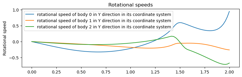
Plot some Angular Speeds.
fig, ax = plt.subplots(figsize=(8, 2.5), layout='constrained')
for i in range(3, 6):
    ax.plot(sys.times, resultat[:, 3*i+1], label='rotational speed of '
               f'body {i - 3} in Y direction in its coordinate system')
ax.set_title('Rotational speeds')
ax.set_ylabel('Rotational speed')
_ = ax.legend()
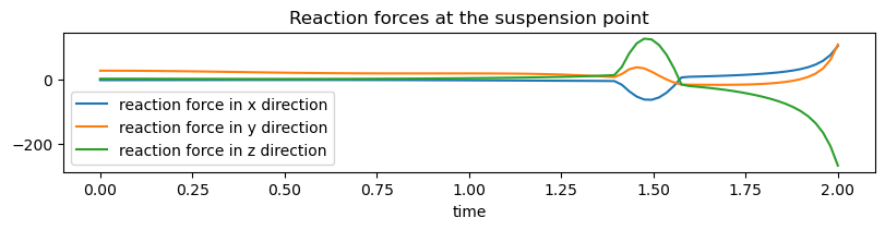
Calculate and plot the reaction forces.
output_results = sys.evaluate_outputs(x=resultat, t=sys.times)

fig, ax = plt.subplots(figsize=(8, 2), layout='constrained')
ax.plot(sys.times, output_results[:, -3],
        label='reaction force in x direction')
ax.set_title('Reaction forces at the suspension point')
ax.plot(sys.times, output_results[:, -2],
        label='reaction force in y direction')
ax.plot(sys.times, output_results[:, -1],
        label='reaction force in z direction')
ax.set_xlabel('time')
_ = ax.legend()
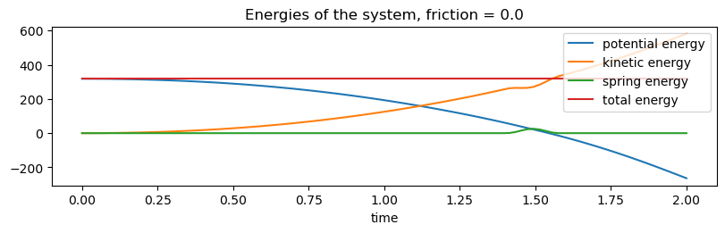
Plot the energies.
fig, ax = plt.subplots(figsize=(8, 2.5), layout='constrained')
ax.plot(sys.times, output_results[:, 0], label='potential energy')
ax.plot(sys.times, output_results[:, 1], label='kinetic energy')
ax.plot(sys.times, output_results[:, 2], label='spring energy')
ax.plot(sys.times, output_results[:, 3], label='total energy')
ax.set_title('Energies of the system, '
             f'friction = {sys.constants[reibung]}')
ax.set_xlabel('time')
ax.legend()

if sys.constants[reibung] == 0.0:
    max_total_energy = max(output_results[:, 3])
    min_total_energy = min(output_results[:, 3])
    delta = (max_total_energy - min_total_energy) / max_total_energy * 100
    print('Max deviation of total energy from being constant: '
          f'{delta:.3e} %')
Max deviation of total energy from being constant: 2.910e-07 %
Animation with PyDy Visualization
groesse is an empirical factor to get the right size of the animation,
found by trial and error.
groesse = 25.0

farben = ['orange', 'blue', 'green', 'red', 'yellow']
viz_frames = []

for i, (ball, point, link) in enumerate(zip(balls, points, links)):
    ball_shape = Sphere(name='sphere{}'.format(i),
                        radius=r,
                        color=farben[i])

    viz_frames.append(VisualizationFrame('ball_frame{}'.format(i),
                                         ball,
                                         ball_shape))

    point_shape = Sphere(name='point{}'.format(i), radius=0.5 / groesse,
                         color='black')

    viz_frames.append(VisualizationFrame('point_frame{}'.format(i),
                                         A[i],
                                         point,
                                         point_shape))

    link_shape = Cylinder(name='cylinder{}'.format(i),
                          radius=0.25 / groesse,
                          length=l,
                          color='red')

    viz_frames.append(VisualizationFrame('link_frame{}'.format(i),
                                         link,
                                         link_shape))

scene = Scene(N, P0, *viz_frames)

scene.times = sys.times
pL_vals_scene = [val / groesse for val in pL_vals]
scene.constants = dict(zip(pL, pL_vals_scene))
scene.states_symbols = q + u

scene.states_trajectories = resultat[:, :-3]

scene.display_jupyter(axes_arrow_length=20)