Carvallo-Whipple Bicycle Model
Note
You can download this example as a Python script:
carvallo-whipple.py or Jupyter notebook:
carvallo-whipple.ipynb.
Warning
This example requires SymPy >= 1.13 due to the use of the Cramer’s rule linear solver.
This example creates a nonlinear model and simulation of the Carvallo-Whipple Bicycle Model ([Carvallo1899], [Whipple1899]). This formulation uses the conventions described in [Moore2012] which are equivalent to the models described in [Meijaard2007] and [Basu-Mandal2007].
Import the necessary libraries, classes, and functions:
import numpy as np
import sympy as sm
import sympy.physics.mechanics as mec
import matplotlib.pyplot as plt
from pydy.system import System
from pydy.viz import Sphere, Cylinder, VisualizationFrame, Scene
System Diagrams
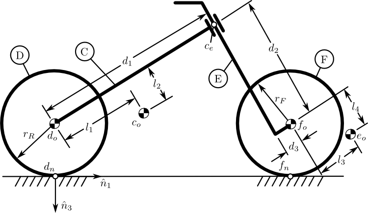
Geometric variable definitions.
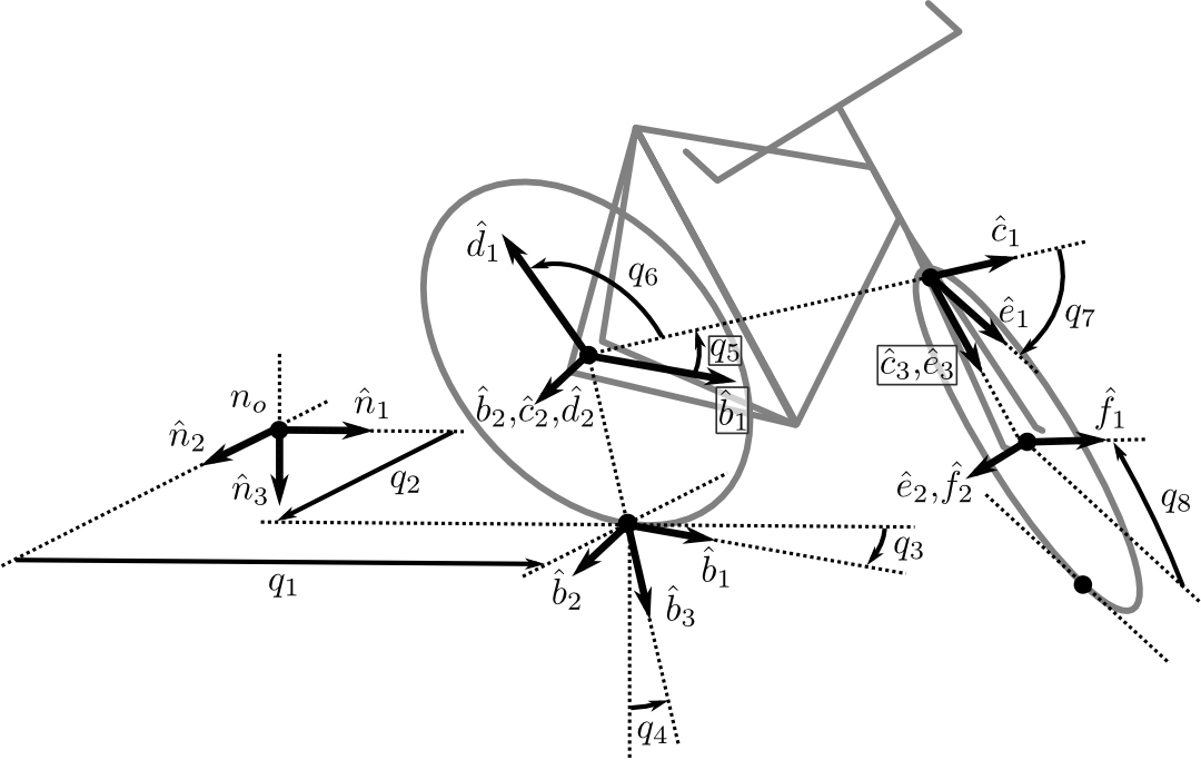
Configuration coordinate definitions.
Reference Frames
Use a reference frame that mimics the notation in [Moore2012].
class ReferenceFrame(mec.ReferenceFrame):
   """Subclass that enforces the desired unit vector indice style."""

   def __init__(self, *args, **kwargs):

      kwargs.pop('indices', None)
      kwargs.pop('latexs', None)

      lab = args[0].lower()
      tex = r'\hat{{{}}}_{}'

      super(ReferenceFrame, self).__init__(*args,
                                             indices=('1', '2', '3'),
                                             latexs=(tex.format(lab, '1'),
                                                   tex.format(lab, '2'),
                                                   tex.format(lab, '3')),
                                             **kwargs)
Define some useful references frames:
\(N\): Newtonian Frame
\(A\): Yaw Frame, auxiliary frame
\(B\): Roll Frame, axillary frame
\(C\): Rear Frame
\(D\): Rear Wheel Frame
\(E\): Front Frame
\(F\): Front Wheel Frame
N = ReferenceFrame('N')
A = ReferenceFrame('A')
B = ReferenceFrame('B')
C = ReferenceFrame('C')
D = ReferenceFrame('D')
E = ReferenceFrame('E')
F = ReferenceFrame('F')
Generalized Coordinates and Speeds
All of the following variables are a functions of time, \(t\).
\(q_1\): perpendicular distance from the \(\hat{n}_2\) axis to the rear contact point in the ground plane
\(q_2\): perpendicular distance from the \(\hat{n}_1\) axis to the rear contact point in the ground plane
\(q_3\): frame yaw angle
\(q_4\): frame roll angle
\(q_5\): frame pitch angle
\(q_6\): front wheel rotation angle
\(q_7\): steering rotation angle
\(q_8\): rear wheel rotation angle
\(q_9\): perpendicular distance from the \(\hat{n}_2\) axis to the front contact point in the ground plane
\(q_{10}\): perpendicular distance from the \(\hat{n}_1\) axis to the front contact point in the ground plane
q1, q2, q3, q4 = mec.dynamicsymbols('q1 q2 q3 q4')
q5, q6, q7, q8 = mec.dynamicsymbols('q5 q6 q7 q8')

u1, u2, u3, u4 = mec.dynamicsymbols('u1 u2 u3 u4')
u5, u6, u7, u8 = mec.dynamicsymbols('u5 u6 u7 u8')
Orientation of Reference Frames
Declare the orientation of each frame to define the yaw, roll, and pitch of the rear frame relative to the Newtonian frame. The define steer of the front frame relative to the rear frame. The wheel rotations are ignorable coordinates and skipped for convenience.
# rear frame yaw
A.orient(N, 'Axis', (q3, N['3']))
# rear frame roll
B.orient(A, 'Axis', (q4, A['1']))
# rear frame pitch
C.orient(B, 'Axis', (q5, B['2']))
# front frame steer
E.orient(C, 'Axis', (q7, C['3']))
Constants
Declare variables that are constant with respect to time for the model’s physical parameters.
\(r_f\): radius of front wheel
\(r_r\): radius of rear wheel
\(d_1\): the perpendicular distance from the steer axis to the center of the rear wheel (rear offset)
\(d_2\): the distance between wheels along the steer axis
\(d_3\): the perpendicular distance from the steer axis to the center of the front wheel (fork offset)
\(l_1\): the distance in the \(\hat{c}_1\) direction from the center of the rear wheel to the frame center of mass
\(l_2\): the distance in the \(\hat{c}_3\) direction from the center of the rear wheel to the frame center of mass
\(l_3\): the distance in the \(\hat{e}_1\) direction from the front wheel center to the center of mass of the fork
\(l_4\): the distance in the \(\hat{e}_3\) direction from the front wheel center to the center of mass of the fork
# geometry
rf, rr = sm.symbols('rf rr')
d1, d2, d3 = sm.symbols('d1 d2 d3')
l1, l2, l3, l4 = sm.symbols('l1 l2 l3 l4')

# acceleration due to gravity
g = sm.symbols('g')

# mass
mc, md, me, mf = sm.symbols('mc md me mf')

# inertia
ic11, ic22, ic33, ic31 = sm.symbols('ic11 ic22 ic33 ic31')
id11, id22 = sm.symbols('id11 id22')
ie11, ie22, ie33, ie31 = sm.symbols('ie11 ie22 ie33 ie31')
if11, if22 = sm.symbols('if11 if22')
Specifieds
Declare three specified torques that are functions of time.
\(T_4\) : roll torque, between Newtonian frame and rear frame
\(T_6\) : rear wheel torque, between rear wheel and rear frame
\(T_7\) : steer torque, between rear frame and front frame
T4, T6, T7 = mec.dynamicsymbols('T4 T6 T7')
Position Vectors
# inertial origin
o = mec.Point('o')

# rear wheel contact point
dn = mec.Point('dn')
dn.set_pos(o, q1*N['1'] + q2*N['2'])

# rear wheel contact point to rear wheel center
do = mec.Point('do')
do.set_pos(dn, -rr * B['3'])

# rear wheel center to bicycle frame center
co = mec.Point('co')
co.set_pos(do, l1 * C['1'] + l2 * C['3'])

# rear wheel center to steer axis point
ce = mec.Point('ce')
ce.set_pos(do, d1 * C['1'])

# steer axis point to the front wheel center
fo = mec.Point('fo')
fo.set_pos(ce, d2 * E['3'] + d3 * E['1'])

# front wheel center to front frame center
eo = mec.Point('eo')
eo.set_pos(fo, l3 * E['1'] + l4 * E['3'])

# locate the point fixed on the wheel which instantaneously touches the
# ground
fn = mec.Point('fn')
fn.set_pos(fo, rf * E['2'].cross(A['3']).cross(E['2']).normalize())
Holonomic Constraint
The front contact point \(f_n\) and the rear contact point \(d_n\) must both reside in the ground plane.
holonomic = fn.pos_from(dn).dot(A['3'])
This expression defines a configuration constraint among \(q_4\), \(q_5\), and \(q_7\).
mec.find_dynamicsymbols(holonomic)
{q4(t), q5(t), q7(t)}
Kinematical Differential Equations
Define the generalized speeds all as \(u=\dot{q}\).
t = mec.dynamicsymbols._t

kinematical = [q1.diff(t) - u1,  # x
               q2.diff(t) - u2,  # y
               q3.diff(t) - u3,  # yaw
               q4.diff(t) - u4,  # roll
               q5.diff(t) - u5,  # pitch
               q7.diff(t) - u7]  # steer
Angular Velocities
A.set_ang_vel(N, u3 * N['3'])  # yaw rate
B.set_ang_vel(A, u4 * A['1'])  # roll rate
C.set_ang_vel(B, u5 * B['2'])  # pitch rate
D.set_ang_vel(C, u6 * C['2'])  # rear wheel rate
E.set_ang_vel(C, u7 * C['3'])  # steer rate
F.set_ang_vel(E, u8 * E['2'])  # front wheel rate
Linear Velocities
# origin is fixed in N
o.set_vel(N, 0*N['1'])

# rear wheel contact stays in ground plane
dn.set_vel(N, u1*N['1'] + u2*N['2'])

# mass centers
do.v2pt_theory(dn, N, C)
co.v2pt_theory(do, N, C)
ce.v2pt_theory(do, N, C)
fo.v2pt_theory(ce, N, E)
eo.v2pt_theory(fo, N, E);  # suppress output
Motion Constraints
Enforce the no slip condition at the rear and front wheel contact point. Also
include an extra motion constraint not allowing vertical motion of the front
contact point. Note that this is an integrable constraint, i.e. the derivative
of nonholonomic above. It is not a nonholonomic constraint, but we include
it because we can’t easy eliminate a dependent generalized coordinate with
nonholonmic.
# wheel contact velocities (for nonholonomic constraints)
N_v_dn = do.vel(N) + D.ang_vel_in(N).cross(dn.pos_from(do))
N_v_fn = fo.vel(N) + F.ang_vel_in(N).cross(fn.pos_from(fo))

nonholonomic = [
    N_v_dn.dot(A['1']),
    N_v_dn.dot(A['2']),
    N_v_fn.dot(A['1']),
    N_v_fn.dot(A['2']),
    N_v_fn.dot(A['3']),
]
Inertia
The inertia dyadics are defined with respect to the rear and front frames.
Ic = mec.inertia(C, ic11, ic22, ic33, 0, 0, ic31)
Id = mec.inertia(C, id11, id22, id11, 0, 0, 0)
Ie = mec.inertia(E, ie11, ie22, ie33, 0, 0, ie31)
If = mec.inertia(E, if11, if22, if11, 0, 0, 0)
Rigid Bodies
rear_frame = mec.RigidBody('Rear Frame', co, C, mc, (Ic, co))
rear_wheel = mec.RigidBody('Rear Wheel', do, D, md, (Id, do))
front_frame = mec.RigidBody('Front Frame', eo, E, me, (Ie, eo))
front_wheel = mec.RigidBody('Front Wheel', fo, F, mf, (If, fo))

bodies = [rear_frame, rear_wheel, front_frame, front_wheel]
Loads
Gravity acts on each rigid body:
# gravity
Fco = (co, mc*g*A['3'])
Fdo = (do, md*g*A['3'])
Feo = (eo, me*g*A['3'])
Ffo = (fo, mf*g*A['3'])
Control torques for the three degrees of freedom:
# input torques
Tc = (C, T4*A['1'] - T6*B['2'] - T7*C['3'])
Td = (D, T6*C['2'])
Te = (E, T7*C['3'])

loads = [Fco, Fdo, Feo, Ffo, Tc, Td, Te]
Baumgarte’s Stabilization
The holonomic constraint, the single algebraic equation in the equations of
motion, will drift during numerical integration. Baumgarte’s stabilization
technique can be used to limit the drift [Baumgarte1972]. This requires
manually setting the acceleration level constraint equations in KanesMethod
with ones that append the Baumgarte force to the holonomic constraint.
acc_constraints = [c.diff(t) for c in nonholonomic]
alpha = sm.symbols('alpha')
acc_constraints[-1] += 2*alpha*nonholonomic[-1] + alpha**2*holonomic
Kane’s Method
Provide all of the kinematic information to KanesMethod, selecting the
three independent generalized speeds. The constraint solver uses the Cramer’s
rule based linear solver to mitigate divide-by-zero issues for the constraint
equations.
kane = mec.KanesMethod(N,
                       [q1, q2, q3, q4, q7],  # x, y, yaw, roll, steer
                       [u4, u6, u7],  # roll rate, rear wheel rate, steer rate
                       kd_eqs=kinematical,
                       q_dependent=[q5],  # pitch angle
                       configuration_constraints=[holonomic],
                       u_dependent=[u1, u2, u3, u5, u8],  # x', y', yaw rate, pitch rate, front wheel rate
                       velocity_constraints=nonholonomic,
                       acceleration_constraints=acc_constraints,
                       constraint_solver='CRAMER')
Provide the rigid bodies and all loads to generate Kane’s equations:
fr, frstar = kane.kanes_equations(bodies, loads)
Simulating the System
PyDy’s System is a wrapper that holds the KanesMethod object to
integrate the equations of motion using numerical values of constants.
sys = System(kane)
Now, we specify the numerical values of the constants and the initial values of states in the form of a dict. The are the benchmark values used in [Meijaard2007] converted to the [Moore2012] formulation.
sys.constants = {
   rf: 0.35,
   rr: 0.3,
   d1: 0.9534570696121849,
   d3: 0.03207142672761929,
   d2: 0.2676445084476887,
   l1: 0.4707271515135145,
   l2: -0.47792881146460797,
   l4: -0.3699518200282974,
   l3: -0.00597083392418685,
   mc: 85.0,
   md: 2.0,
   me: 4.0,
   mf: 3.0,
   id11: 0.0603,
   id22: 0.12,
   if11: 0.1405,
   if22: 0.28,
   ic11: 7.178169776497895,
   ic22: 11.0,
   ic31: 3.8225535938357873,
   ic33: 4.821830223502103,
   ie11: 0.05841337700152972,
   ie22: 0.06,
   ie31: 0.009119225261946298,
   ie33: 0.007586622998470264,
   g: 9.81,
   alpha: 10.0,
}
Generate a time vector over which the integration will be carried out.
fps = 30  # frames per second
duration = 10.0  # seconds
sys.times = np.linspace(0.0, duration, num=int(duration*fps))
The trajectory of the states over time can be found by calling the
.integrate() method. But due to the complexity of the equations of motion
it is helpful to use the cython generator for faster numerical evaluation
and the symbolic linear solver can also be set to maximize performance as well
as avoid divide-by-zero issues.
_ = sys.generate_ode_function(generator='cython',
                              linear_sys_solver='sympy:CRAMER')
Setup the initial conditions such that the bicycle is traveling at some forward speeds and has an initial positive roll rate.
initial_speed = 4.6  # m/s
initial_roll_rate = 0.5  # rad/s
pitch_guess = np.deg2rad(20.0)
wheel_speed_guess = -initial_speed/0.3
Set all of the initial conditions and provide guesses for dependent coordinates and speeds.
sys.initial_conditions = {q1: 0.0,
                          q2: 0.0,
                          q3: 0.0,
                          q4: 0.0,
                          q5: pitch_guess,
                          q7: 0.0,
                          u1: initial_speed,
                          u2: 0.0,
                          u3: 0.0,
                          u4: initial_roll_rate,
                          u5: 0.0,
                          u6: wheel_speed_guess,
                          u7: 0.0,
                          u8: wheel_speed_guess}
Solve for the dependent states given the values of the independent states and guesses for the dependent states.
sys.set_dependent_initial_conditions(dep_vars=(q5, u2, u3, u5, u6, u8))
sys.initial_conditions
{q1(t): 0.0,
 q2(t): 0.0,
 q3(t): 0.0,
 q4(t): 0.0,
 q5(t): np.float64(0.31415926535897915),
 q7(t): 0.0,
 u1(t): 4.6,
 u2(t): np.float64(0.0),
 u3(t): np.float64(5.4422697285546875e-17),
 u4(t): 0.5,
 u5(t): np.float64(-0.0),
 u6(t): np.float64(-15.333333333333332),
 u7(t): 0.0,
 u8(t): np.float64(-13.142857142857142)}
Check if the initial conditions satisfy the constraints.
np.isclose(sys.evaluate_constraints(), 0.0)
array([ True, True, True, True, True])
Test that the initial condition gives a valid result.
sys.evaluate_ode()
array([ 4.60000000e+00,  0.00000000e+00,  5.44226973e-17,  5.00000000e-01,
        0.00000000e+00, -0.00000000e+00, -2.42701635e-01, -4.66261635e-14,
        8.45665204e+00,  1.39878491e-14,  2.50344408e-16,  6.30804237e-01,
        1.65686912e-14, -3.99652830e-14])
Now integrate the equations of motion through time.
x_trajectory = sys.integrate()
xdot_trajectory = sys.evaluate_ode(x=x_trajectory)
Evaluate the constraints at each time value.
con_trajectory = sys.evaluate_constraints(x=x_trajectory)
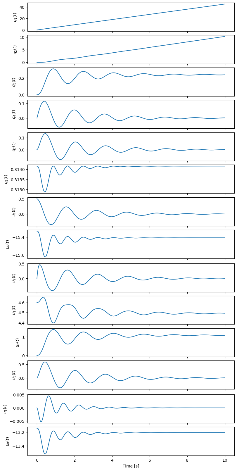
Plot the Trajectories
State trajectories:
fig, axes = plt.subplots(len(sys.states), 1, sharex=True,
                         layout='constrained')
fig.set_size_inches(8, 16)
for ax, traj, s in zip(axes, x_trajectory.T, sys.states):
    ax.plot(sys.times, traj)
    ax.set_ylabel(sm.latex(s, mode='inline'))
axes[-1].set_xlabel('Time [s]');
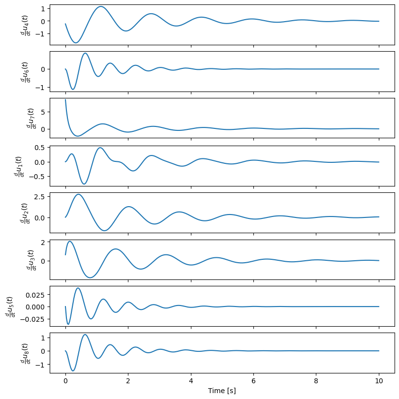
Acceleration trajectories:
fig, axes = plt.subplots(len(sys.speeds), 1, sharex=True,
                         layout='constrained')
fig.set_size_inches(8, 8)
for ax, traj, s in zip(axes, xdot_trajectory.T[6:], sys.speeds):
    ax.plot(sys.times, traj)
    ax.set_ylabel(sm.latex(s.diff(), mode='inline'))
axes[-1].set_xlabel('Time [s]');
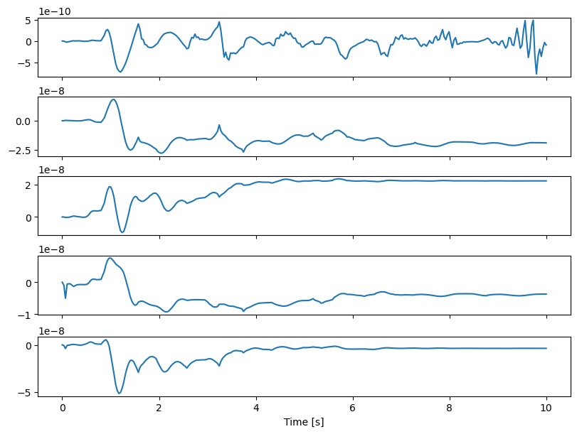
Constraint trajectories:
fig, axes = plt.subplots(con_trajectory.shape[1], 1,
                         sharex=True,
                         layout='constrained')
fig.set_size_inches(8, 6)
for ax, traj in zip(axes, con_trajectory.T):
    ax.plot(sys.times, traj)
axes[-1].set_xlabel('Time [s]');
Visualizing the System Motion
Create two cylinders to represent the front and rear wheels.
rear_wheel_circle = Cylinder(radius=sys.constants[rr], length=0.01,
                             color="green", name='rear wheel')
front_wheel_circle = Cylinder(radius=sys.constants[rf], length=0.01,
                              color="green", name='front wheel')
rear_wheel_vframe = VisualizationFrame(B, do, rear_wheel_circle)
front_wheel_vframe = VisualizationFrame(E, fo, front_wheel_circle)
Create some cylinders to represent the front and rear frames.
d1_cylinder = Cylinder(radius=0.02, length=sys.constants[d1],
                       color='black', name='rear frame d1')
d2_cylinder = Cylinder(radius=0.02, length=sys.constants[d2],
                       color='black', name='front frame d2')
d3_cylinder = Cylinder(radius=0.02, length=sys.constants[d3],
                       color='black', name='front frame d3')

d1_frame = VisualizationFrame(C.orientnew('C_r', 'Axis', (sm.pi/2, C.z)),
                              do.locatenew('d1_half', d1/2*C.x), d1_cylinder)
d2_frame = VisualizationFrame(E.orientnew('E_r', 'Axis', (-sm.pi/2, E.x)),
                              fo.locatenew('d2_half', -d3*E.x - d2/2*E.z), d2_cylinder)
d3_frame = VisualizationFrame(E.orientnew('E_r', 'Axis', (sm.pi/2, E.z)),
                              fo.locatenew('d3_half', -d3/2*E.x), d3_cylinder)
Create some spheres to represent the mass centers of the front and rear frames.
co_sphere = Sphere(radius=0.05, color='blue', name='rear frame co')
eo_sphere = Sphere(radius=0.05, color='blue', name='rear frame eo')
co_frame = VisualizationFrame(C, co, co_sphere)
eo_frame = VisualizationFrame(E, eo, eo_sphere)
Create the scene and add the visualization frames.
scene = Scene(N, o, system=sys)
scene.visualization_frames = [front_wheel_vframe, rear_wheel_vframe,
                              d1_frame, d2_frame, d3_frame,
                              co_frame, eo_frame]
Now, call the display method.
scene.display_jupyter(axes_arrow_length=5.0)
References
Whipple, Francis J. W. “The Stability of the Motion of a Bicycle.” Quarterly Journal of Pure and Applied Mathematics 30 (1899): 312–48.
Carvallo, E. Théorie Du Mouvement Du Monocycle et de La Bicyclette. Paris, France: Gauthier- Villars, 1899.
Baumgarte, J. (1972). Stabilization of Constraints and Integrals of Motion in Dynamical Systems. Computer Methods in Applied Mechanics and Engineering, 1, 1–16.
Basu-Mandal, Pradipta, Anindya Chatterjee, and J.M Papadopoulos. “Hands-Free Circular Motions of a Benchmark Bicycle.” Proceedings of the Royal Society A: Mathematical, Physical and Engineering Sciences 463, no. 2084 (August 8, 2007): 1983–2003. https://doi.org/10.1098/rspa.2007.1849.
Meijaard, J. P., Jim M. Papadopoulos, Andy Ruina, and A. L. Schwab. “Linearized Dynamics Equations for the Balance and Steer of a Bicycle: A Benchmark and Review.” Proceedings of the Royal Society A: Mathematical, Physical and Engineering Sciences 463, no. 2084 (August 8, 2007): 1955–82.
Moore, Jason K. “Human Control of a Bicycle.” Doctor of Philosophy, University of California, 2012. http://moorepants.github.io/dissertation.