Multi Degree of Freedom Holonomic System
Note
You can download this example as a Python script:
multidof-holonomic.py or Jupyter notebook:
multidof-holonomic.ipynb.
Problem Description
This is an example of a holonomic system that includes both particles and rigid bodies with contributing forces and torques, some of which are specified forces and torques.
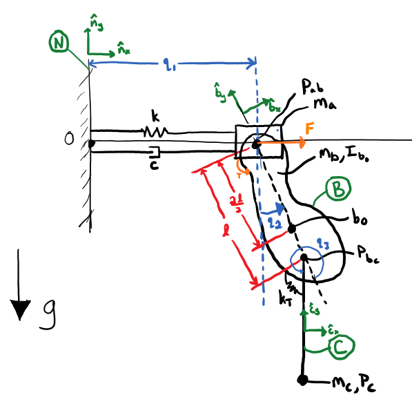
Generalized coordinates:
\(q_1\): Lateral distance of block from wall.
\(q_2\): Angle of the compound pendulum from vertical.
\(q_3\): Angle of the simple pendulum from the compound pendulum.
Generalized speeds:
\(u_1 = \dot{q}_1\): Lateral speed of block.
\(u_2 = {}^N\bar{v}^{Bo} \cdot \hat{b}_x\)
\(u_3 = \dot{q}_3\): Angular speed of C relative to B.
The block and the bob of the simple pendulum are modeled as particles and \(B\) is a rigid body.
Loads:
gravity acts on \(B\) and \(P_c\).
a linear spring and damper act on \(P_{ab}\)
a rotational linear spring acts on \(C\) relative to \(B\)
specified torque \(T\) acts on \(B\) relative to \(N\)
specified force \(F\) acts on \(P_{ab}\)
import sympy as sm
import sympy.physics.mechanics as me
me.init_vprinting()
Generalized coordinates
q1, q2, q3 = me.dynamicsymbols('q1, q2, q3')
Generalized speeds
u1, u2, u3 = me.dynamicsymbols('u1, u2, u3')
Specified Inputs
F, T = me.dynamicsymbols('F, T')
Constants
k, c, ma, mb, mc, IB_bo, l, kT, g = sm.symbols('k, c, m_a, m_b, m_c, I_{B_bo}, l, k_T, g')
k, c, ma, mb, mc, IB_bo, l, kT, g

Reference Frames
N = me.ReferenceFrame('N')
B = N.orientnew('B', 'Axis', (q2, N.z))
C = B.orientnew('C', 'Axis', (q3, N.z))
Points
O = me.Point('O')
Pab = O.locatenew('P_{ab}', q1 * N.x)
Bo = Pab.locatenew('B_o', - 2 * l / 3 * B.y)
Pbc = Pab.locatenew('P_{bc}', -l * B.y)
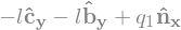
Pc = Pbc.locatenew('P_c', -l * C.y)
Pc.pos_from(O)
Linear Velocities
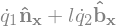
Pab.set_vel(N, Pab.pos_from(O).dt(N))
Pab.vel(N)

Bo.v2pt_theory(Pab, N, B)

Pbc.v2pt_theory(Pab, N, B)
Pc.v2pt_theory(Pbc, N, C)
Kinematic Differential Equations
One non-trivial generalized speed definition is used.
u1_eq = sm.Eq(u1, Pab.vel(N).dot(N.x))
u2_eq = sm.Eq(u2, Bo.vel(N).dot(B.x))
u3_eq = sm.Eq(u3, C.ang_vel_in(B).dot(B.z))
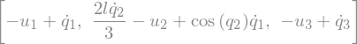
qdots = sm.solve([u1_eq, u2_eq, u3_eq], q1.diff(), q2.diff(), q3.diff())
qdots
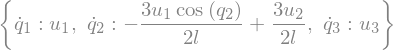
Substitute expressions for the \(\dot{q}\)‘s.
Pab.set_vel(N, Pab.vel(N).subs(qdots).simplify())
Pab.vel(N)

Bo.set_vel(N, Bo.vel(N).subs(qdots).express(B).simplify())
Bo.vel(N)
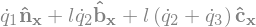
Pc.set_vel(N, Pc.vel(N).subs(qdots).simplify())
Pc.vel(N)

Angular Velocities
B.set_ang_vel(N, B.ang_vel_in(N).subs(qdots).simplify())
B.ang_vel_in(N)
C.set_ang_vel(B, u3 * N.z)
C.ang_vel_in(N)
Mass and Inertia
ma, mc

IB = me.inertia(B, 0, 0, IB_bo)
IB
Loads (forces and torques)
Make sure these are defined in terms of the q’s and u’s.
Rab = (F - k*q1 - c*qdots[q1.diff()]) * N.x
Rab
Rbo = -(mb*g)*N.y
Rbo

Rc = -(mc*g)*N.y
Rc

TB = (T + kT*q3)*N.z
TB
Equal and opposite torque on \(C\) from \(B\).
TC = -kT*q3*N.z
TC

Kane’s Equations
kdes = [u1_eq.rhs - u1_eq.lhs,
        u2_eq.rhs - u2_eq.lhs,
        u3_eq.rhs - u3_eq.lhs]
kdes
block = me.Particle('block', Pab, ma)
pendulum = me.RigidBody('pendulum', Bo, B, mb, (IB, Bo))
bob = me.Particle('bob', Pc, mc)

bodies = [block, pendulum, bob]
Loads are a list of (force, point) or reference (frame, torque) 2-tuples:
loads = [(Pab, Rab),
         (Bo, Rbo),
         (Pc, Rc),
         (B, TB),
         (C, TC)]
kane = me.KanesMethod(N, (q1, q2, q3), (u1, u2, u3), kd_eqs=kdes)
fr, frstar = kane.kanes_equations(bodies, loads=loads)
Simulation
from pydy.system import System
import numpy as np  # provides basic array types and some linear algebra
import matplotlib.pyplot as plt  # used for plots
sys = System(kane)
Define numerical values for each constant using a dictionary. Make sure units are compatible!
sys.constants = {ma: 1.0,  # kg
                 mb: 2.0,  # kg
                 mc: 1.0,  # kg
                 g: 9.81,  # m/s/s
                 l: 2.0,  # m
                 IB_bo: 2.0,  # kg*m**2
                 c: 10.0,  # kg/s
                 k: 60.0,  # N/m
                 kT: 10.0}  # N*m/rad
Provide an array of monotonic values of time that you’d like the state values reported at.
sys.times = np.linspace(0.0, 20.0, num=500)
Set the initial conditions for each state.
sys.states

sys.initial_conditions = {q1: 1.0,  # m
                          q2: 0.0,  # rad
                          q3: 0.0,  # rad
                          u1: 0.0,  # m/s
                          u2: 0.0,  # rad/s
                          u3: 0.0}  # rad/s
There are several ways that the specified force and torque can be provided to the system. Here are three options, the last one is actually used.
A single value can be provided to set the force and torque to be constant.
specifieds = {F: 0.0,  # N
              T: 1.0}  # N*m
The same thing as 1) can be done using an array.
specifieds = {(F, T): np.array([0.0, 1.0])}
3) A numerical function can be defined to calculate the input at a specific time.
def sin_f(x, t):
    """Returns the force F given the state vector x and time value t.

    Parameters
    ==========
    x : ndarray, shape(n,)
        The states in the order specified in System.states.
    t : float
        The value of time.

    Returns
    =======
    float
        The value of the force at time t.

    """
    return 1.0 * np.sin(2 * np.pi * t)

specifieds = {F: sin_f,  # N
              T: 1.0}  # N*m
A single numerical function can also be used for both.
def sin_f_t(x, t):
    return  np.array([5.0 * np.sin(2.0 * np.pi * t),
                      10.0 * np.cos(2.0 * np.pi * t)])

specifieds = {(F, T): sin_f_t}
sys.specifieds = specifieds
Integrate the equations of motion and get the state trajectories x:
x = sys.integrate()
x.shape

Plot Results
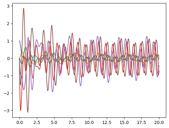
plt.plot(sys.times, x);
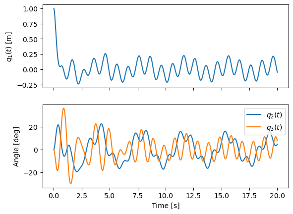
fig, axes = plt.subplots(2, 1, sharex=True)
axes[0].plot(sys.times, x[:, 0])
axes[0].set_ylabel('{} [m]'.format(sm.latex(q1, mode='inline')))
axes[1].plot(sys.times, np.rad2deg(x[:, 1:3]))
axes[1].legend([sm.latex(q, mode='inline') for q in (q2, q3)])
axes[1].set_xlabel('Time [s]')
axes[1].set_ylabel('Angle [deg]');
Animate with PyDy and pythreejs
from pydy.viz.shapes import Cube, Cylinder, Sphere, Plane
from pydy.viz.visualization_frame import VisualizationFrame
from pydy.viz import Scene
Define some PyDy shapes for each moving object you want visible in the scene. Each shape needs a unique name with no spaces.
block_shape = Cube(0.25, color='azure', name='block')
cpendulum_shape = Plane(l, l/4, color='mediumpurple', name='cpendulum')
spendulum_shape = Cylinder(l, 0.02, color='azure', name='spendulum')
bob_shape = Sphere(0.2, color='mediumpurple', name='bob')
Create a visualization frame that attaches a shape to a reference frame and point. Note that the center of the plane and cylinder for the two pendulums is at its geometric center, so two new points are created so that the position of those points are calculated instead of the mass centers, which are not at the geometric centers.
v1 = VisualizationFrame('block', N, Pab, block_shape)

v2 = VisualizationFrame('cpendulum',
                        B,
                        Pab.locatenew('Bc', -l/2*B.y),
                        cpendulum_shape)

v3 = VisualizationFrame('spendulum',
                        C,
                        Pbc.locatenew('Cc', -l/2*C.y),
                        spendulum_shape)

v4 = VisualizationFrame('bob', C, Pc, bob_shape)
Create a scene with the origin point O and base reference frame N and
the fully defined System.
scene = Scene(N, O, v1, v2, v3, v4, system=sys)
Make sure pythreejs is installed and then call display_jupyter for a
3D animation of the system.
scene.display_jupyter(axes_arrow_length=1.0)
It is then fairly simple to change constants, initial conditions,
simulation time, or specified inputs and visualize the effects. Below
the lateral spring is stretched more initially and when
display_jupyter() is called the system equations are integrated with
the new initial condition.
sys.initial_conditions[q1] = 5.0 # m
scene.display_jupyter(axes_arrow_length=1.0)