Linear Mass-Spring-Damper with Gravity
Note
You can download this example as a Python script:
mass-spring-damper.py or Jupyter notebook:
mass-spring-damper.ipynb.
Defining the Problem
Here we will derive the equations of motion for the classic mass-spring-damper system under the influence of gravity. The following figure gives a pictorial description of the problem.

Start by loading in the core functionality of both SymPy and Mechanics.
import sympy as sm
import sympy.physics.mechanics as me
We can make use of the pretty printing of our results by loading SymPy’s printing extension, in particular we will use the vector printing which is nice for mechanics objects.
me.init_vprinting()
We’ll start by defining the variables we will need for this problem:
\(x(t)\): distance of the particle from the ceiling
\(v(t)\): speed of the particle
\(m\): mass of the particle
\(c\): damping coefficient of the damper
\(k\): stiffness of the spring
\(g\): acceleration due to gravity
\(t\): time
x, v = me.dynamicsymbols('x v')
m, c, k, g, t = sm.symbols('m c k g t')
Now, we define a Newtonian reference frame that represents the ceiling which the particle is attached to, \(C\).
ceiling = me.ReferenceFrame('C')
We will need two points, one to represent the original position of the particle which stays fixed in the ceiling frame, \(O\), and the second one, \(P\) which is aligned with the particle as it moves.
O = me.Point('O')
P = me.Point('P')
The velocity of point \(O\) in the ceiling is zero.
O.set_vel(ceiling, 0)
Point \(P\) can move downward in the \(y\) direction and its velocity is specified as \(v\) in the downward direction.
P.set_pos(O, x * ceiling.x)
P.set_vel(ceiling, v * ceiling.x)
P.vel(ceiling)

There are three forces acting on the particle. Those due to the acceleration of gravity, the damper, and the spring.
damping = -c * P.vel(ceiling)
stiffness = -k * P.pos_from(O)
gravity = m * g * ceiling.x
forces = damping + stiffness + gravity
forces

Now we can use Newton’s second law, \(0=F-ma\), to form the equation of motion of the system.
zero = me.dot(forces - m * P.acc(ceiling), ceiling.x)
zero

We can then form the first order equations of motion by solving for \(\frac{dv}{dt}\) and introducing the kinematical differential equation, \(v=\frac{dx}{dt}\).
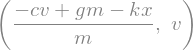
dv_by_dt = sm.solve(zero, v.diff(t))[0]
dx_by_dt = v
dv_by_dt, dx_by_dt
Forming the equations of motion can also be done with the automated methods
available in the Mechanics package: LagrangesMethod and KanesMethod.
Here we will make use of Kane’s method to find the same equations of motion
that we found manually above. First, define a particle that represents the mass
attached to the damper and spring.
mass = me.Particle('mass', P, m)
Now we can construct a KanesMethod object by passing in the generalized
coordinate, \(x\), the generalized speed, \(v\), and the kinematical
differential equation which relates the two, \(0=v-\frac{dx}{dt}\).
kane = me.KanesMethod(ceiling, q_ind=[x], u_ind=[v], kd_eqs=[v - x.diff(t)])
Now Kane’s equations can be computed, and we can obtain \(F_r\) and \(F_r^*\).
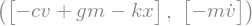
fr, frstar = kane.kanes_equations([mass], loads=[(P, forces)])
fr, frstar
The equations are also available in the form \(M\frac{d}{dt}[q,u]^T=f(q, u)\) and we can extract the mass matrix, \(M\), and the forcing functions, \(f\).
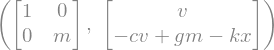
M = kane.mass_matrix_full
f = kane.forcing_full
M, f
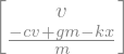
Finally, we can form the first order differential equations of motion \(\frac{d}{dt}[q,u]^T=M^{-1}f(\dot{u}, u, q)\), which is the same as previously found.
M.inv() * f
Simulating the system
Now that we have defined the mass-spring-damper system, we are going to simulate it.
PyDy’s System is a wrapper that holds the Kanes object to integrate the
equations of motion using numerical values of constants.
from pydy.system import System
sys = System(kane)
Now, we specify the numerical values of the constants and the initial values of states in the form of a dict.
sys.constants = {m:10.0, g:9.8, c:5.0, k:10.0}
sys.initial_conditions = {x:0.0, v:0.0}
We must generate a time vector over which the integration will be carried out.
NumPy’s linspace is often useful for this.
from numpy import linspace
fps = 60
duration = 10.0
sys.times = linspace(0.0, duration, num=int(duration*fps))
The trajectory of the states over time can be found by calling the
.integrate() method.
x_trajectory = sys.integrate()
Visualizing the System
PyDy has a native module pydy.viz which is used to visualize a System in an
interactive 3D GUI.
from pydy.viz import *
For visualizing the system, we need to create shapes for the objects we wish to
visualize, and map each of them to a VisualizationFrame, which holds the
position and orientation of the object. First create a sphere to represent the
bob and attach it to the point \(P\) and the ceiling reference frame (the
sphere does not rotate with respect to the ceiling).
bob = Sphere(2.0, color="red", name='bob')
bob_vframe = VisualizationFrame(ceiling, P, bob)
Now create a circular disc that represents the ceiling and fix it to the ceiling reference frame. The circle’s default axis is aligned with its local \(z\) axis, so we need to attach it to a rotated ceiling reference frame if we want the circle’s axis to align with the \(\hat{c}_x\) unit vector.
ceiling_circle = Circle(radius=10, color="white", name='ceiling')
rotated = ceiling.orientnew("C_R", 'Axis', [sm.pi/2, ceiling.y])
ceiling_vframe = VisualizationFrame(rotated, O, ceiling_circle)
Now we initialize a Scene. A Scene contains all the information required to
visualize a System onto a canvas. It takes a ReferenceFrame and Point as
arguments.
scene = Scene(ceiling, O, system=sys)
We provide the VisualizationFrames, which we want to visualize as a list to scene.
scene.visualization_frames = [bob_vframe, ceiling_vframe]
Now, we call the display method.
scene.display_jupyter(axes_arrow_length=5.0)